

US States by Cost of Living in 2026: Latest 2025 Annual Snapshot
How U.S. State Price Levels Compare Using the Latest MERIC Annual Average
Information updated: May 3, 2026
The cost of living index compares everyday prices across U.S. states and selected jurisdictions against a national baseline of 100. A score below 100 means a place is less expensive than the U.S. average; a score above 100 means it is more expensive. The ranking is useful for salary comparisons, relocation decisions, retirement planning, housing affordability checks and state-level economic context.
The source table is MERIC Cost of Living Data Series, Annual Average 2025. The figures are not a 2026 forecast. They are the latest complete annual benchmark available at the time of update and should be read under the 2025 Annual Average data label until a complete 2026 annual average is published.
Continue exploring
More StatRanker rankings on wages, income, housing costs and affordability.
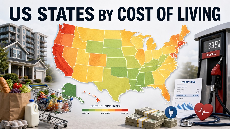
Overview: the low-cost cluster is mostly inland, while the high-cost cluster is coastal or island-based
The lowest-cost group is concentrated in the South and Midwest. Oklahoma, Mississippi, West Virginia, Alabama, Kansas and Missouri all sit below 89 on the composite index, meaning their broad basket of prices is more than 11% cheaper than the U.S. average. Housing is the clearest separating factor: the housing index for many low-cost states is in the high 60s to high 70s, far below the national baseline.
The expensive end of the distribution is shaped by housing scarcity, island logistics, coastal land constraints and high-income metro concentration. Hawaii is the clear outlier with a composite index of 183.9 and a housing index of 299.0. Massachusetts, California and the District of Columbia also stand far above the national average, while New York and Alaska form the next tier of high-cost living.
What the lowest-cost group shows
The Top 20 lowest-cost entries are dominated by states where housing remains well below the U.S. average. Several of them have grocery, transportation and health care values close to the national baseline, so the overall affordability advantage is not uniform across every category.
Why the ranking matters
A nominal salary can mislead if price levels differ sharply by state. An income that feels comfortable in Oklahoma or Missouri may not buy the same housing, utilities or services in Hawaii, California, Massachusetts or D.C.
Top 10 lowest-cost U.S. states in the MERIC annual average
Rank 1 means the lowest composite cost of living in the MERIC source table. The Top 10 is not a list of the highest-income or best-value states; it is a ranking of relative price levels compared with the U.S. average.
| Rank | State | Composite index | Housing index |
|---|---|---|---|
| 1 | Oklahoma | 84.7 | 68.8 |
| 2 | Mississippi | 86.0 | 71.6 |
| 3 | West Virginia | 88.0 | 71.2 |
| 4 | Alabama | 88.1 | 71.2 |
| 5 | Kansas | 88.4 | 76.9 |
| 6 | Missouri | 88.9 | 77.5 |
| 7 | Iowa | 89.8 | 77.7 |
| 8 | Arkansas | 90.1 | 78.8 |
| 9 | Tennessee | 90.1 | 82.4 |
| 10 | Indiana | 90.7 | 75.4 |
Top 10 lowest-cost states from MERIC / C2ER Annual Average 2025. Index values are relative to U.S. average = 100.
Chart: most expensive states and jurisdictions by cost of living index
The expensive end of the ranking is more spread out than the affordable end. Hawaii is structurally separate from the rest of the field because island logistics and housing costs push the composite index far above the mainland range.
Bar width is scaled to Hawaii = 100% within this chart. The index itself uses U.S. average = 100, so every value above 100 is more expensive than the national average.
Chart data fallback
Highest composite indexes: Hawaii 183.9; Massachusetts 148.5; California 143.1; District of Columbia 137.8; Alaska 126.7; New York 125.8; Maryland 117.4; New Jersey 115.3; Maine 114.0; Connecticut 114.0.
Full ranking: U.S. states and jurisdictions by cost of living index
The table ranks places from lowest to highest composite cost of living. Use the controls to search, sort, filter by region, filter by cost band, or switch the value cell from index to percentage difference versus the U.S. average.
Showing 52 rows.
| Rank | State / jurisdiction | Cost index | Housing index |
|---|---|---|---|
| 1 | Oklahoma | 84.7−15.3% | 68.8 |
| 2 | Mississippi | 86.0−14.0% | 71.6 |
| 3 | West Virginia | 88.0−12.0% | 71.2 |
| 4 | Alabama | 88.1−11.9% | 71.2 |
| 5 | Kansas | 88.4−11.6% | 76.9 |
| 6 | Missouri | 88.9−11.1% | 77.5 |
| 7 | Iowa | 89.8−10.2% | 77.7 |
| 8 | Arkansas | 90.1−9.9% | 78.8 |
| 9 | Tennessee | 90.1−9.9% | 82.4 |
| 10 | Indiana | 90.7−9.3% | 75.4 |
| 11 | Texas | 91.1−8.9% | 79.4 |
| 12 | North Dakota | 91.1−8.9% | 75.7 |
| 13 | Kentucky | 91.5−8.5% | 74.8 |
| 14 | Nebraska | 91.8−8.2% | 78.7 |
| 15 | South Dakota | 91.8−8.2% | 85.9 |
| 16 | Michigan | 91.9−8.1% | 78.3 |
| 17 | Georgia | 92.2−7.8% | 79.7 |
| 18 | South Carolina | 92.7−7.3% | 80.6 |
| 19 | Louisiana | 92.9−7.1% | 84.5 |
| 20 | Minnesota | 93.6−6.4% | 80.6 |
| 21 | New Mexico | 93.7−6.3% | 88.6 |
| 22 | Wyoming | 94.6−5.4% | 87.1 |
| 23 | Ohio | 94.6−5.4% | 87.6 |
| 24 | Illinois | 95.0−5.0% | 84.3 |
| 25 | Montana | 96.8−3.2% | 94.4 |
| 26 | Pennsylvania | 97.1−2.9% | 86.8 |
| 27 | North Carolina | 97.9−2.1% | 94.0 |
| 28 | Wisconsin | 98.5−1.5% | 99.0 |
| 29 | Idaho | 99.3−0.7% | 100.3 |
| 30 | Utah | 99.5−0.5% | 108.8 |
| 31 | Nevada | 99.7−0.3% | 110.7 |
| 32 | Florida | 101.4+1.4% | 103.5 |
| 33 | Puerto Rico | 102.1+2.1% | 99.1 |
| 34 | Virginia | 102.2+2.2% | 106.7 |
| 35 | Delaware | 103.1+3.1% | 102.3 |
| 36 | Colorado | 103.1+3.1% | 108.8 |
| 37 | Arizona | 110.3+10.3% | 127.3 |
| 38 | New Hampshire | 110.5+10.5% | 115.6 |
| 39 | Rhode Island | 110.7+10.7% | 115.1 |
| 40 | Oregon | 112.8+12.8% | 127.4 |
| 41 | Washington | 112.9+12.9% | 118.3 |
| 42 | Vermont | 113.5+13.5% | 129.0 |
| 43 | Connecticut | 114.0+14.0% | 122.3 |
| 44 | Maine | 114.0+14.0% | 135.7 |
| 45 | New Jersey | 115.3+15.3% | 141.9 |
| 46 | Maryland | 117.4+17.4% | 141.3 |
| 47 | New York | 125.8+25.8% | 174.7 |
| 48 | Alaska | 126.7+26.7% | 123.6 |
| 49 | District of Columbia | 137.8+37.8% | 204.7 |
| 50 | California | 143.1+43.1% | 199.4 |
| 51 | Massachusetts | 148.5+48.5% | 221.0 |
| 52 | Hawaii | 183.9+83.9% | 299.0 |
MERIC / C2ER Annual Average 2025. Unit: composite cost of living index, U.S. average = 100. Difference vs U.S. is calculated as index minus 100. Information updated: May 3, 2026.
Methodology
The ranking uses the MERIC Cost of Living Data Series for Annual Average 2025. MERIC derives state-level cost of living values from participating cities and metropolitan areas in the C2ER Cost of Living Index survey. The composite index is built from six major categories: grocery items, housing, utilities, transportation, health care, and miscellaneous goods and services. The U.S. average is fixed at 100, so values can be interpreted directly as percent distance from the national average.
The table is sorted from the lowest composite index to the highest composite index. The data label remains Annual Average 2025 because a complete 2026 annual average cannot exist before the year is complete. The correct status is latest complete annual benchmark, not estimate or forecast.
Values are shown to one decimal place, matching the source format. The full source ranking includes 52 entries: 50 states, the District of Columbia and Puerto Rico. Region labels are added for filtering and are not part of the original index calculation. The main table keeps four columns to maintain readability: rank, place, composite index and housing index. Housing is included because it explains a large part of the spread between low-cost and high-cost states.
The index should not be read as a city-level relocation quote or a household budget. It reflects participating urban areas within each state and does not capture every county, rural area or neighborhood. Small differences between nearby index values should be interpreted cautiously. For public policy, salary benchmarking or relocation decisions, this index is best combined with income data, local rent data, BEA Regional Price Parities and BLS price-change measures.
Insights from the state cost of living ranking
Housing separates the ranking more than groceries
Grocery indexes vary, but the largest gaps come from housing. Oklahoma, West Virginia, Alabama and Mississippi have housing indexes close to 70, while Massachusetts, D.C., California and Hawaii are near or above 200. That difference changes the real value of wages, pensions and savings.
The South and Midwest dominate the affordable end
Most of the first 20 positions are states from the South or Midwest. Their advantage is not always a lower price for every category, but the combined effect of cheaper housing and generally moderate costs across transportation, utilities and miscellaneous spending.
The expensive cluster is geographically specific
Hawaii and Alaska face location and logistics costs. California, New York, Massachusetts, New Jersey, Maryland and D.C. face high housing costs around dense labor markets and constrained land. The result is a high-cost cluster that is not evenly distributed across the country.
Near-average states can still hide pressure points
A state near 100 is not necessarily affordable for every household. Utah and Nevada sit close to the national average on the composite index, but their housing indexes are above 108 and 110. That matters more for renters and homebuyers than for households with stable housing costs.
What the ranking means for readers
For workers comparing job offers, the index helps translate nominal pay into real purchasing power. A higher salary in a high-cost state may not mean a higher standard of living once rent, mortgage payments, utilities, commuting and services are included. For remote workers, the same income can stretch very differently depending on whether the household lives in a low-cost state such as Oklahoma or a high-cost market such as Hawaii, Massachusetts or California.
For retirees and households on fixed income, the ranking highlights why state selection can affect the durability of savings. Low-cost states may reduce monthly pressure, but taxes, health care access, insurance, climate risk and family proximity still matter. For employers, the table can support location-based compensation analysis, but it should be used with occupation wages, local labor-market conditions and housing-market data rather than as a single pay formula.
For policymakers, the contrast between composite and housing indexes is especially important. A state can appear near the national average overall while still having housing pressure that weakens affordability for first-time buyers, renters and young families. Cost of living is therefore not only a consumer issue; it affects migration, workforce attraction, regional competitiveness and household formation.
FAQ
Does a cost of living index of 84.7 mean Oklahoma is 84.7% cheaper than the U.S. average?
No. The U.S. average is 100. Oklahoma’s index of 84.7 means its composite cost level is about 15.3% below the U.S. average, not 84.7% below it.
Why is the article labeled 2026 if the data year is 2025?
The ranking uses the latest complete annual data available. A full-year 2026 annual average cannot be available until after 2026 ends, so the data label is Annual Average 2025.
Is this the same as inflation?
No. The cost of living index compares price levels across places at a point in time. Inflation measures price changes over time. A state can be expensive but have slow inflation, or relatively affordable but experience fast price increases.
Why does housing matter so much in the ranking?
Housing is one of the largest household expenses and varies sharply by state and metro area. The housing index ranges from below 70 in some low-cost states to nearly 300 in Hawaii, making it the most visible driver of the overall spread.
Can this ranking decide where someone should move?
It can narrow the comparison, but it should not be the only input. A practical relocation decision also depends on wages, job security, taxes, insurance, commuting, schools, health care access, climate exposure and the exact city or county.
Why are District of Columbia and Puerto Rico included?
They appear in the MERIC source table, so they are included for transparency. The row count is therefore 52, not 50. The table labels them as jurisdictions rather than states.
Sources
The ranking uses the latest complete annual state-level cost of living table available from MERIC and C2ER. Federal sources are included for price-level and inflation context, not as replacements for the MERIC ranking.
-
Missouri Economic Research and Information Center — Cost of Living Data Series
Primary source for the 2025 Annual Average state and jurisdiction ranking used in the table.
https://meric.mo.gov/data/cost-living-data-series -
Council for Community and Economic Research — Cost of Living Index methodology
Methodological reference for the C2ER composite index and its major component categories.
https://c2c.coli.org/compare.asp?action=methodology -
U.S. Bureau of Economic Analysis — Regional Price Parities by State and Metro Area
Federal source for state and metro price-level comparisons; useful for validating broad geographic cost differences.
https://www.bea.gov/data/prices-inflation/regional-price-parities-state-and-metro-area -
U.S. Bureau of Labor Statistics — Consumer Price Index
Federal source for measuring price changes over time; included to distinguish inflation from cost-of-living level comparisons.
https://www.bls.gov/cpi/
Related rankings
More StatRanker rankings on wages, income, housing costs and affordability.
Inflation Rate by Country: IMF 2025 Estimates and Latest WEO Observations
Open rankingCountries by Gasoline Price, 2026: Top 100 Most Expensive Countries for Gasoline
Open rankingUS States by Electricity Prices, 2026 Snapshot
Open rankingTop 100 Countries by Inflation Rate (Consumer Prices), Latest Year
Open rankingStatRanker (Website)
administrator